Top Open Datasets for Deep Learning

Introduction

The key to getting better at deep learning (or most fields in life) is practice. Practice on a variety of problems – from image processing to speech recognition. Each of these problem has it’s own unique nuance and approach.

But where can you get this data? A lot of research papers you see these days use proprietary datasets that are usually not released to the general public. This becomes a problem, if you want to learn and apply your newly acquired skills.

If you have faced this problem, we have a solution for you. We have curated a list of openly available datasets for your perusal.

In this article, we have listed a collection of high quality datasets that every deep learning enthusiast should work on to apply and improve their skillset. Working on these datasets will make you a better data scientist and the amount of learning you will have will be invaluable in your career. We have also included papers with state-of-the-art (SOTA) results for you to go through and improve your models.

How to use these datasets?

First things first – these datasets are huge in size! So make sure you have a fast internet connection with no / very high limit on the amount of data you can download.

There are numerous ways how you can use these datasets. You can use them to apply various Deep Learning techniques. You can use them to hone your skills, understand how to identify and structure each problem, think of unique use cases and publish your findings for everyone to see!

The datasets are divided into three categories – Image Processing, Natural Language Processing, and Audio/Speech Processing.

Let’s dive into it!

Image Datasets

MNIST

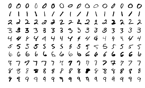
MNIST is one of the most popular deep learning datasets out there. It’s a dataset of handwritten digits and contains a training set of 60,000 examples and a test set of 10,000 examples. It’s a good database for trying learning techniques and deep recognition patterns on real-world data while spending minimum time and effort in data preprocessing.

Size: ~50 MB

Number of Records: 70,000 images in 10 classes

SOTA: Dynamic Routing Between Capsules

MS-COCO

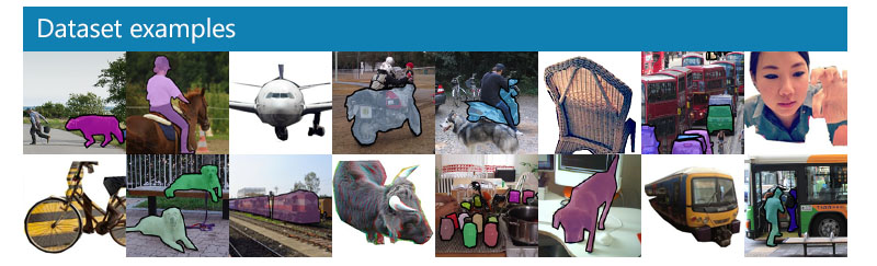
COCO is a large-scale and rich for object detection, segmentation and captioning dataset. It has several features:

• Object segmentation
• Recognition in context
• Superpixel stuff segmentation
• 330K images (>200K labeled)
• 1.5 million object instances
• 80 object categories
• 91 stuff categories
• 5 captions per image
• 250,000 people with keypoints

Size: ~25 GB (Compressed)

Number of Records: 330K images, 80 object categories, 5 captions per image, 250,000 people with key points

SOTA : Mask R-CNN

ImageNet

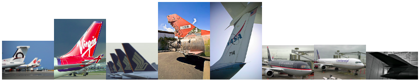
ImageNet is a dataset of images that are organized according to the WordNet hierarchy. WordNet contains approximately 100,000 phrases and ImageNet has provided around 1000 images on average to illustrate each phrase.

Size: ~150GB

Number of Records: Total number of images: ~1,500,000; each with multiple bounding boxes and respective class labels

SOTA : Aggregated Residual Transformations for Deep Neural Networks

Open Images Dataset

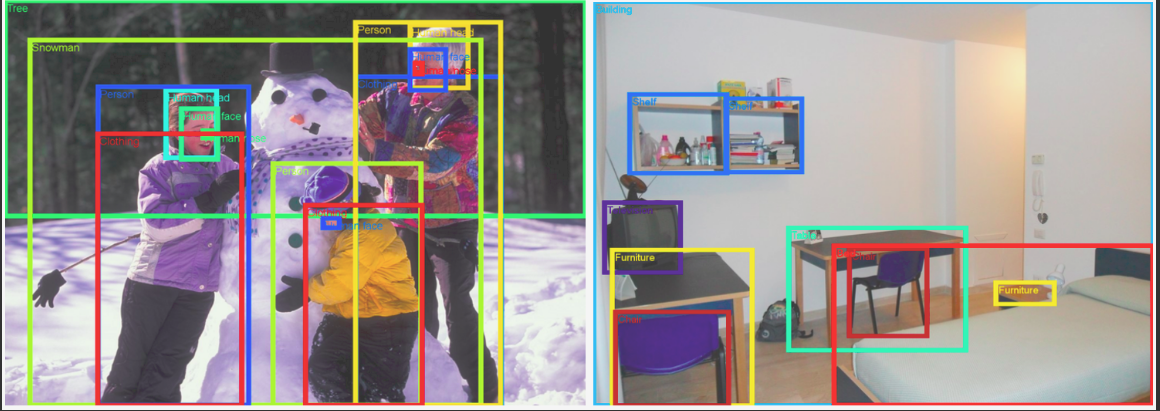
Open Images is a dataset of almost 9 million URLs for images. These images have been annotated with image-level labels bounding boxes spanning thousands of classes. The dataset contains a training set of 9,011,219 images, a validation set of 41,260 images and a test set of 125,436 images.

Size: 500 GB (Compressed)

Number of Records: 9,011,219 images with more than 5k labels

SOTA : Resnet 101 image classification model (trained on V2 data): Model checkpoint, Checkpoint readme, Inference code.

VisualQA

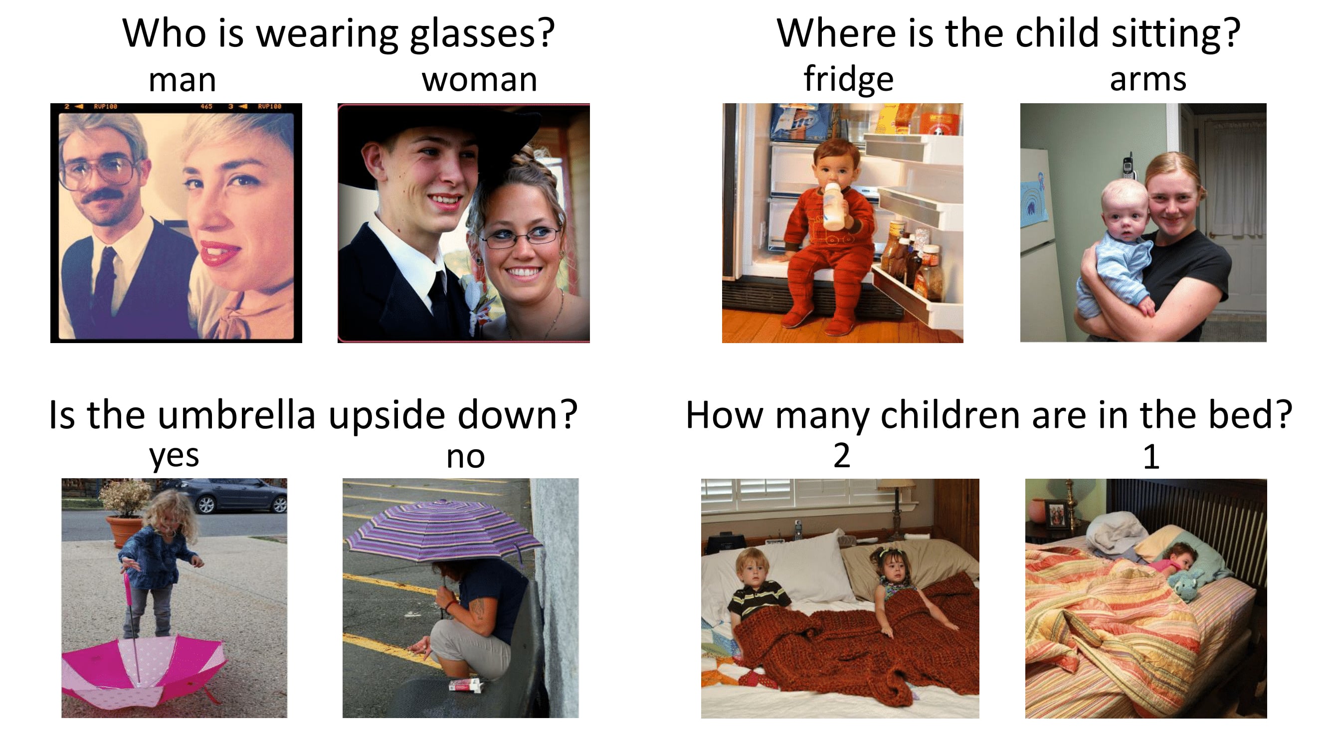
VQA is a dataset containing open-ended questions about images. These questions require an understanding of vision and language. Some of the interesting features of this dataset are:

• 265,016 images (COCO and abstract scenes)
• At least 3 questions (5.4 questions on average) per image
• 10 ground truth answers per question
• 3 plausible (but likely incorrect) answers per question
• Automatic evaluation metric

Size: 25 GB (Compressed)

Number of Records: 265,016 images, at least 3 questions per image, 10 ground truth answers per question

SOTA : Tips and Tricks for Visual Question Answering: Learnings from the 2017 Challenge

The Street View House Numbers (SVHN)

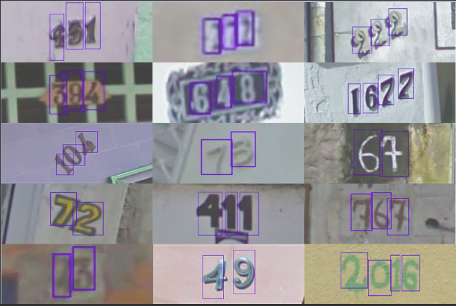
This is a real-world image dataset for developing object detection algorithms. This requires minimum data preprocessing. It is similar to the MNIST dataset mentioned in this list, but has more labelled data (over 600,000 images). The data has been collected from house numbers viewed in Google Street View.

Size: 2.5 GB

Number of Records: 6,30,420 images in 10 classes

SOTA : Distributional Smoothing With Virtual Adversarial Training

CIFAR-10

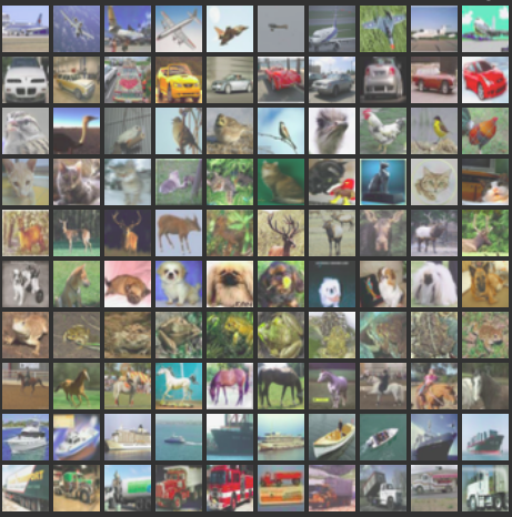
This dataset is another one for image classification. It consists of 60,000 images of 10 classes (each class is represented as a row in the above image). In total, there are 50,000 training images and 10,000 test images. The dataset is divided into 6 parts – 5 training batches and 1 test batch. Each batch has 10,000 images.

Size: 170 MB

Number of Records: 60,000 images in 10 classes

SOTA : ShakeDrop regularization

Fashion-MNIST

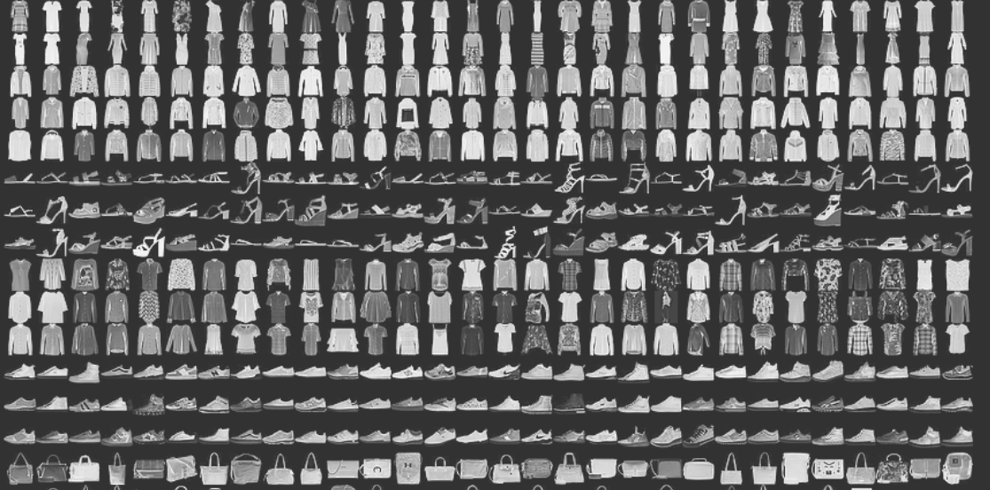
Fashion-MNIST consists of 60,000 training images and 10,000 test images. It is a MNIST-like fashion product database. The developers believe MNIST has been overused so they created this as a direct replacement for that dataset. Each image is in greyscale and associated with a label from 10 classes.

Size: 30 MB

Number of Records: 70,000 images in 10 classes

SOTA : Random Erasing Data Augmentation

Natural Language Processing

IMDB Reviews

This is a dream dataset for movie lovers. It is meant for binary sentiment classification and has far more data than any previous datasets in this field. Apart from the training and test review examples, there is further unlabeled data for use as well. Raw text and preprocessed bag of words formats have also been included.

Size: 80 MB

Number of Records: 25,000 highly polar movie reviews for training, and 25,000 for testing

SOTA : Learning Structured Text Representations

Twenty Newsgroups

This dataset, as the name suggests, contains information about newsgroups. To curate this dataset, 1000 Usenet articles were taken from 20 different newsgroups. The articles have typical features like subject lines, signatures, and quotes.

Size: 20 MB

Number of Records: 20,000 messages taken from 20 newsgroups

SOTA : Very Deep Convolutional Networks for Text Classification,

Sentiment140

Sentiment140 is a dataset that can be used for sentiment analysis. A popular dataset, it is perfect to start off your NLP journey. Emotions have been pre-removed from the data. The final dataset has the below 6 features:

• polarity of the tweet
• id of the tweet
• date of the tweet
• the query
• username of the tweeter
• text of the tweet

Size: 80 MB (Compressed)

Number of Records: 1,60,000 tweets

SOTA : Assessing State-of-the-Art Sentiment Models on State-of-the-Art Sentiment Datasets

WordNet

Mentioned in the ImageNet dataset above, WordNet is a large database of English synsets. Synsets are groups of synonyms that each describe a different concept. WordNet’s structure makes it a very useful tool for NLP.

Size: 10 MB

Number of Records: 117,000 synsets is linked to other synsets by means of a small number of “conceptual relations.

SOTA : Wordnets: State of the Art and Perspectives

Yelp Reviews

This is an open dataset released by Yelp for learning purposes. It consists of millions of user reviews, businesses attributes and over 200,000 pictures from multiple metropolitan areas. This is a very commonly used dataset for NLP challenges globally.

Size: 2.66 GB JSON, 2.9 GB SQL and 7.5 GB Photos (all compressed)

Number of Records: 5,200,000 reviews, 174,000 business attributes, 200,000 pictures and 11 metropolitan areas

SOTA : Attentive Convolution

The Wikipedia Corpus

This dataset is a collection of a the full text on Wikipedia. It contains almost 1.9 billion words from more than 4 million articles. What makes this a powerful NLP dataset is that you search by word, phrase or part of a paragraph itself.

Size: 20 MB

Number of Records: 4,400,000 articles containing 1.9 billion words

SOTA : Breaking The Softmax Bottelneck: A High-Rank RNN language Model

The Blog Authorship Corpus

This dataset consists of blog posts collected from thousands of bloggers and has been gathered from blogger.com. Each blog is provided as a separate file. Each blog contains a minimum of 200 occurrences of commonly used English words.

Size: 300 MB

Number of Records: 681,288 posts with over 140 million words

SOTA : Character-level and Multi-channel Convolutional Neural Networks for Large-scale Authorship Attribution

Machine Translation of Various Languages

This dataset consists of training data for four European languages. The task here is to improve the current translation methods. You can participate in any of the following language pairs:

• English-Chinese and Chinese-English
• English-Czech and Czech-English
• English-Estonian and Estonian-English
• English-Finnish and Finnish-English
• English-German and German-English
• English-Kazakh and Kazakh-English
• English-Russian and Russian-English
• English-Turkish and Turkish-English

Size: ~15 GB

Number of Records: ~30,000,000 sentences and their translations

SOTA : Attention Is All You Need

Audio/Speech Datasets

Free Spoken Digit Dataset

Another entry in this list for inspired by the MNIST dataset! This one was created to solve the task of identifying spoken digits in audio samples. It’s an open dataset so the hope is that it will keep growing as people keep contributing more samples. Currently, it contains the below characteristics:

• 3 speakers
• 1,500 recordings (50 of each digit per speaker)
• English pronunciations

Size: 10 MB

Number of Records: 1,500 audio samples

SOTA : Raw Waveform-based Audio Classification Using Sample-level CNN Architectures

Free Music Archive (FMA)

FMA is a dataset for music analysis. The dataset consists of full-length and HQ audio, pre-computed features, and track and user-level metadata. It an an open dataset created for evaluating several tasks in MIR. Below is the list of csv files the dataset has along with what they include:

• tracks.csv: per track metadata such as ID, title, artist, genres, tags and play counts, for all 106,574 tracks.
• genres.csv: all 163 genre IDs with their name and parent (used to infer the genre hierarchy and top-level genres).
• features.csv: common features extracted with librosa.
• echonest.csv: audio features provided by Echonest (now Spotify) for a subset of 13,129 tracks.

Size: ~1000 GB

Number of Records: ~100,000 tracks

SOTA : Learning to Recognize Musical Genre from Audio

Ballroom

This dataset contains ballroom dancing audio files. A few characteristic excerpts of many dance styles are provided in real audio format. Below are a few characteristics of the dataset:

• Total number of instances: 698
• Duration: ~30 s
• Total duration: ~20940 s

Size: 14GB (Compressed)

Number of Records: ~700 audio samples

SOTA : A Multi-Model Approach To Beat Tracking Considering Heterogeneous Music Styles

Million Song Dataset

The Million Song Dataset is a freely-available collection of audio features and metadata for a million contemporary popular music tracks. Its purposes are:

• To encourage research on algorithms that scale to commercial sizes
• To provide a reference dataset for evaluating research
• As a shortcut alternative to creating a large dataset with APIs (e.g. The Echo Nest’s)
• To help new researchers get started in the MIR field

The core of the dataset is the feature analysis and metadata for one million songs. The dataset does not include any audio, only the derived features. The sample audio can be fetched from services like7digital, using code provided by Columbia University.

Size: 280 GB

Number of Records: PS – its a million songs!

SOTA :  Preliminary Study on a Recommender System for the Million Songs Dataset Challenge

LibriSpeech

This dataset is a large-scale corpus of around 1000 hours of English speech. The data has been sourced from audiobooks from the LibriVox project. It has been segmented and aligned properly. If you’re looking for a starting point, check out already prepared Acoustic models that are trained on this data set at kaldi-asr.org and language models, suitable for evaluation, at http://www.openslr.org/11/.

Size: ~60 GB

Number of Records: 1000 hours of speech

SOTA : Letter-Based Speech Recognition with Gated ConvNets

VoxCeleb

VoxCeleb is a large-scale speaker identification dataset. It contains around 100,000 utterances by 1,251 celebrities, extracted from YouTube videos. The data is mostly gender balanced (males comprise of 55%). The celebrities span a diverse range of accents, professions and age. There is no overlap between the development and test sets. It’s an intriguing use case for isolating and identifying which superstar the voice belongs to.

Size: 150 MB

Number of Records: 100,000 utterances by 1,251 celebrities

SOTA : VoxCeleb: a large-scale speaker identification dataset

Analytics Vidhya Practice Problems

For your practice, we also provide real life problems and datasets to get your hands dirty. In this section, we’ve listed down the deep learning practice problems on our DataHack platform.

Twitter Sentiment Analysis

Hate Speech in the form of racism and sexism has become a nuisance on twitter and it is important to segregate these sort of tweets from the rest. In this Practice problem, we provide Twitter data that has both normal and hate tweets. Your task as a Data Scientist is to identify the tweets which are hate tweets and which are not.

Size: 3 MB

Number of Records: 31,962 tweets

Age Detection of Indian Actors

This is a fascinating challenge for any deep learning enthusiast. The dataset contains thousands of images of Indian actors and your task is to identify their age. All the images are manually selected and cropped from the video frames resulting in a high degree of variability interms of scale, pose, expression, illumination, age, resolution, occlusion, and makeup.

Size: 48 MB (Compressed)

Number of Records: 19,906 images in the training set and 6636 in the test set

SOTA: Hands on with Deep Learning – Solution for Age Detection Practice Problem

Urban Sound Classification

This dataset consists of more than 8000 sound excerpts of urban sounds from 10 classes. This practice problem is meant to introduce you to audio processing in the usual classification scenario.

Size: Training set – 3 GB (Compressed), Test set – 2 GB (Compressed)

Number of Records: 8732 labeled sound excerpts (<=4s) of urban sounds from 10 classes

Top Open Datasets For Machine Learning

When working with comprehensive datasets every data scientist seems to have their favorite go to. For free resources, Mansi Singhal CEO of qplum pointed to data.gov, Socrata, Amazon OpenData, Google public data, Kaggle, and UCI Machine Learning Archives as a few examples. “In financial services industry, we find FRED database incredibly useful,” she said.

Then there are those datasets that are proprietary. “A good example is the stock price data for which you might need to work with an exchange or one of the 3rd party providers,” she said. “For business purposes, there is not much work around and these days exchanges make more money from selling data instead of trading fees.”

But for machine learning, the bigger the better — and that usually translates into large public domain datasets. Either way Singhal said, the key “is to build the in-house tech infrastructure so that you have a pipeline to pull the data, clean and process it and repeat this process periodically without too much overhead.”

With machine learning on the uptick we've done the leg work for you and assembled a list of top public domain datasets as ranked by Github. The full list, along with several other lists of datasets, can be found here. 

• Amazon -This registry is meant to help people discover and share datasets that are available via AWS resources.
• Archive.org Datasets - The dataset collection consists of large data archives from both sites and individuals.
• Archive-it from Internet ArchiveA web archiving service for cultural heritage on the web
• CMU JASA data archive - This is a jasadata archive containing contributed datasets from articles published in the Journal of the American Statistical Association.
• CMU StatLab collections - These are interesting dataset, or collection of data from books.
• Data.World - A public benefit corporation that is focused on creating collaborative open datasets.
• Enigma Public - Billed as “the world’s broadest collection of public data,” is a data management and intelligence company that provides a repository of public data.
• Google - Google’s collection of public datasets.
• KDNuggets Data Collections - Provides datasets for data mining and data science.
• Microsoft Data Science for Research - Microsoft Research’s collection of free datasets, tools and resources.

Random Forest for Beginners

Random Forest is a trademark term for an ensemble of decision trees. In Random Forest, we’ve collection of decision trees (so known as “Forest”). To classify a new object based on attributes, each tree gives a classification and we say the tree “votes” for that class. The forest chooses the classification having the most votes (over all the trees in the forest).

Each tree is planted & grown as follows:

1. If the number of cases in the training set is N, then sample of N cases is taken at random but with replacement. This sample will be the training set for growing the tree.
2. If there are M input variables, a number m<<M is specified such that at each node, m variables are selected at random out of the M and the best split on these m is used to split the node. The value of m is held constant during the forest growing.
3. Each tree is grown to the largest extent possible. There is no pruning.

Python

#Import Library
from sklearn.ensemble import RandomForestClassifier
#Assumed you have, X (predictor) and Y (target) for training data set and x_test(predictor) of test_dataset
# Create Random Forest object
model= RandomForestClassifier()
# Train the model using the training sets and check score
model.fit(X, y)
#Predict Output
predicted= model.predict(x_test)

K-Means for Beginners

It is a type of unsupervised algorithm which  solves the clustering problem. Its procedure follows a simple and easy  way to classify a given data set through a certain number of  clusters (assume k clusters). Data points inside a cluster are homogeneous and heterogeneous to peer groups.

Remember figuring out shapes from ink blots? k means is somewhat similar this activity. You look at the shape and spread to decipher how many different clusters / population are present!

How K-means forms cluster:

1. K-means picks k number of points for each cluster known as centroids.
2. Each data point forms a cluster with the closest centroids i.e. k clusters.
3. Finds the centroid of each cluster based on existing cluster members. Here we have new centroids.
4. As we have new centroids, repeat step 2 and 3. Find the closest distance for each data point from new centroids and get associated with new k-clusters. Repeat this process until convergence occurs i.e. centroids does not change.

How to determine value of K:

In K-means, we have clusters and each cluster has its own centroid. Sum of square of difference between centroid and the data points within a cluster constitutes within sum of square value for that cluster. Also, when the sum of square values for all the clusters are added, it becomes total within sum of square value for the cluster solution.

We know that as the number of cluster increases, this value keeps on decreasing but if you plot the result you may see that the sum of squared distance decreases sharply up to some value of k, and then much more slowly after that. Here, we can find the optimum number of cluster.

Python Code

#Import Library
from sklearn.cluster import KMeans
#Assumed you have, X (attributes) for training data set and x_test(attributes) of test_dataset
# Create KNeighbors classifier object model 
k_means = KMeans(n_clusters=3, random_state=0)
# Train the model using the training sets and check score
model.fit(X)
#Predict Output
predicted= model.predict(x_test)

kNN (k- Nearest Neighbors) for Beginners

It can be used for both classification and regression problems. However, it is more widely used in classification problems in the industry. K nearest neighbors is a simple algorithm that stores all available cases and classifies new cases by a majority vote of its k neighbors. The case being assigned to the class is most common amongst its K nearest neighbors measured by a distance function.

These distance functions can be Euclidean, Manhattan, Minkowski and Hamming distance. First three functions are used for continuous function and fourth one (Hamming) for categorical variables. If K = 1, then the case is simply assigned to the class of its nearest neighbor. At times, choosing K turns out to be a challenge while performing kNN modeling.

More: Introduction to k-nearest neighbors : Simplified.

KNN can easily be mapped to our real lives. If you want to learn about a person, of whom you have no information, you might like to find out about his close friends and the circles he moves in and gain access to his/her information!

Things to consider before selecting kNN:

• KNN is computationally expensive
• Variables should be normalized else higher range variables can bias it
• Works on pre-processing stage more before going for kNN like outlier, noise removal

Python Code

#Import Library
from sklearn.neighbors import KNeighborsClassifier
#Assumed you have, X (predictor) and Y (target) for training data set and x_test(predictor) of test_dataset
# Create KNeighbors classifier object model 
KNeighborsClassifier(n_neighbors=6) # default value for n_neighbors is 5
# Train the model using the training sets and check score
model.fit(X, y)
#Predict Output
predicted= model.predict(x_test)

Naive Bayes for Beginners

It is a classification technique based on Bayes’ theorem with an assumption of independence between predictors. In simple terms, a Naive Bayes classifier assumes that the presence of a particular feature in a class is unrelated to the presence of any other feature. For example, a fruit may be considered to be an apple if it is red, round, and about 3 inches in diameter. Even if these features depend on each other or upon the existence of the other features, a naive Bayes classifier would consider all of these properties to independently contribute to the probability that this fruit is an apple.

Naive Bayesian model is easy to build and particularly useful for very large data sets. Along with simplicity, Naive Bayes is known to outperform even highly sophisticated classification methods.

Bayes theorem provides a way of calculating posterior probability P(c|x) from P(c), P(x) and P(x|c). Look at the equation below:

Here,

• P(c|x) is the posterior probability of class (target) given predictor (attribute). 
• P(c) is the prior probability of class. 
• P(x|c) is the likelihood which is the probability of predictor given class. 
• P(x) is the prior probability of predictor.

Example: Let’s understand it using an example. Below I have a training data set of weather and corresponding target variable ‘Play’. Now, we need to classify whether players will play or not based on weather condition. Let’s follow the below steps to perform it.

Step 1: Convert the data set to frequency table

Step 2: Create Likelihood table by finding the probabilities like Overcast probability = 0.29 and probability of playing is 0.64.

Step 3: Now, use Naive Bayesian equation to calculate the posterior probability for each class. The class with the highest posterior probability is the outcome of prediction.

Problem: Players will pay if weather is sunny, is this statement is correct?

We can solve it using above discussed method, so P(Yes | Sunny) = P( Sunny | Yes) * P(Yes) / P (Sunny)

Here we have P (Sunny |Yes) = 3/9 = 0.33, P(Sunny) = 5/14 = 0.36, P( Yes)= 9/14 = 0.64

Now, P (Yes | Sunny) = 0.33 * 0.64 / 0.36 = 0.60, which has higher probability.

Naive Bayes uses a similar method to predict the probability of different class based on various attributes. This algorithm is mostly used in text classification and with problems having multiple classes.

Python Code

#Import Library
from sklearn.naive_bayes import GaussianNB
#Assumed you have, X (predictor) and Y (target) for training data set and x_test(predictor) of test_dataset
# Create SVM classification object model = GaussianNB() # there is other distribution for multinomial classes like Bernoulli Naive Bayes, Refer link
# Train the model using the training sets and check score
model.fit(X, y)
#Predict Output
predicted= model.predict(x_test)

Support Vector Machine for Beginners

The first time I heard the name “Support Vector Machine”, I felt, if the name itself sounds so complicated the formulation of the concept will be beyond my understanding. Luckily, I saw a few university lecture videos and realized how easy and effective this tool was. In this article, we will talk about how support vector machine works. This article is suitable for readers who do not know much about this algorithm and have a curiosity to learn a new technique. In following articles we will explore the technique in detail and analyze cases where such techniques are stronger than other techniques.

What is a classification analysis?

Let’s consider an example to understand these concepts. We have a population composed of 50%-50% Males and Females. Using a sample of this population, you want to create some set of rules which will guide us the gender class for rest of the population. Using this algorithm, we intend to build a robot which can identify whether a person is a Male or a Female. This is a sample problem of classification analysis. Using some set of rules, we will try to classify the population into two possible segments. For simplicity, let’s assume that the two differentiating factors identified are : Height of the individual and Hair Length. Following is a scatter plot of the sample.

The blue circles in the plot represent females and green squares represents male. A few expected insights from the graph are :

1. Males in our population have a higher average height.

2. Females in our population have longer scalp hairs.

If we were to see an individual with height 180 cms and hair length 4 cms, our best guess will be to classify this individual as a male. This is how we do a classification analysis.

What is a Support Vector and what is SVM?

Support Vectors are simply the co-ordinates of individual observation. For instance, (45,150) is a support vector which corresponds to a female. Support Vector Machine is a frontier which best segregates the Male from the Females. In this case, the two classes are well separated from each other, hence it is easier to find a SVM.

How to find the Support Vector Machine for case in hand?

There are many possible frontier which can classify the problem in hand. Following are the three possible frontiers.

How do we decide which is the best frontier for this particular problem statement?

The easiest way to interpret the objective function in a SVM is to find the minimum distance of the frontier from closest support vector (this can belong to any class). For instance, orange frontier is closest to blue circles. And the closest blue circle is 2 units away from the frontier. Once we have these distances for all the frontiers, we simply choose the frontier with the maximum distance (from the closest support vector). Out of the three shown frontiers, we see the black frontier is farthest from nearest support vector (i.e. 15 units).

What if we do not find a clean frontier which segregates the classes?

Our job was relatively easier finding the SVM in this business case. What if the distribution looked something like as follows :

In such cases, we do not see a straight line frontier directly in current plane which can serve as the SVM. In such cases, we need to map these vector to a higher dimension plane so that they get segregated from each other. Such cases will be covered once we start with the formulation of SVM. For now, you can visualize that such transformation will result into following type of SVM.

Each of the green square in original distribution is mapped on a transformed scale. And transformed scale has clearly segregated classes.

Decision Tree for Beginners

This is one of my favorite algorithm and I use it quite frequently. It is a type of supervised learning algorithm that is mostly used for classification problems. Surprisingly, it works for both categorical and continuous dependent variables. In this algorithm, we split the population into two or more homogeneous sets. This is done based on most significant attributes/ independent variables to make as distinct groups as possible. For more details, you can read: Decision Tree Simplified.

source: statsexchange

In the image above, you can see that population is classified into four different groups based on multiple attributes to identify ‘if they will play or not’. To split the population into different heterogeneous groups, it uses various techniques like Gini, Information Gain, Chi-square, entropy.

The best way to understand how decision tree works, is to play Jezzball – a classic game from Microsoft (image below). Essentially, you have a room with moving walls and you need to create walls such that maximum area gets cleared off with out the balls.

So, every time you split the room with a wall, you are trying to create 2 different populations with in the same room. Decision trees work in very similar fashion by dividing a population in as different groups as possible.

More: Simplified Version of Decision Tree Algorithms

Python Code

#Import Library
#Import other necessary libraries like pandas, numpy...
from sklearn import tree
#Assumed you have, X (predictor) and Y (target) for training data set and x_test(predictor) of test_dataset
# Create tree object 
model = tree.DecisionTreeClassifier(criterion='gini') # for classification, here you can change the algorithm as gini or entropy (information gain) by default it is gini  
# model = tree.DecisionTreeRegressor() for regression
# Train the model using the training sets and check score
model.fit(X, y)
model.score(X, y)
#Predict Output
predicted= model.predict(x_test)

Logistic Regression for Beginners

Don’t get confused by its name! It is a classification not a regression algorithm. It is used to estimate discrete values ( Binary values like 0/1, yes/no, true/false ) based on given set of independent variable(s). In simple words, it predicts the probability of occurrence of an event by fitting data to a logit function. Hence, it is also known as logit regression. Since, it predicts the probability, its output values lies between 0 and 1 (as expected).

Again, let us try and understand this through a simple example.

Let’s say your friend gives you a puzzle to solve. There are only 2 outcome scenarios – either you solve it or you don’t. Now imagine, that you are being given wide range of puzzles / quizzes in an attempt to understand which subjects you are good at. The outcome to this study would be something like this – if you are given a trignometry based tenth grade problem, you are 70% likely to solve it. On the other hand, if it is grade fifth history question, the probability of getting an answer is only 30%. This is what Logistic Regression provides you.

Coming to the math, the log odds of the outcome is modeled as a linear combination of the predictor variables.

odds= p/ (1-p) = probability of event occurrence / probability of not event occurrence
ln(odds) = ln(p/(1-p))
logit(p) = ln(p/(1-p)) = b0+b1X1+b2X2+b3X3....+bkXk

Above, p is the probability of presence of the characteristic of interest. It chooses parameters that maximize the likelihood of observing the sample values rather than that minimize the sum of squared errors (like in ordinary regression).

Now, you may ask, why take a log? For the sake of simplicity, let’s just say that this is one of the best mathematical way to replicate a step function. I can go in more details, but that will beat the purpose of this article.

Python Code

#Import Library
from sklearn.linear_model import LogisticRegression
#Assumed you have, X (predictor) and Y (target) for training data set and x_test(predictor) of test_dataset
# Create logistic regression object
model = LogisticRegression()
# Train the model using the training sets and check score
model.fit(X, y)
model.score(X, y)
#Equation coefficient and Intercept
print('Coefficient: \n', model.coef_)
print('Intercept: \n', model.intercept_)
#Predict Output
predicted= model.predict(x_test)

Linear Regression for beginners

It is used to estimate real values (cost of houses, number of calls, total sales etc.) based on continuous variable(s). Here, we establish relationship between independent and dependent variables by fitting a best line. This best fit line is known as regression line and represented by a linear equation Y= a *X + b.

The best way to understand linear regression is to relive this experience of childhood. Let us say, you ask a child in fifth grade to arrange people in his class by increasing order of weight, without asking them their weights! What do you think the child will do? He / she would likely look (visually analyze) at the height and build of people and arrange them using a combination of these visible parameters. This is linear regression in real life! The child has actually figured out that height and build would be correlated to the weight by a relationship, which looks like the equation above.

In this equation:

• Y – Dependent Variable
• a – Slope
• X – Independent variable
• b – Intercept

These coefficients a and b are derived based on minimizing the sum of squared difference of distance between data points and regression line.

Look at the below example. Here we have identified the best fit line having linear equation y=0.2811x+13.9. Now using this equation, we can find the weight, knowing the height of a person.

Linear Regression is of mainly two types: Simple Linear Regression and Multiple Linear Regression. Simple Linear Regression is characterized by one independent variable. And, Multiple Linear Regression(as the name suggests) is characterized by multiple (more than 1) independent variables. While finding best fit line, you can fit a polynomial or curvilinear regression. And these are known as polynomial or curvilinear regression.

Python Code

#Import Library
#Import other necessary libraries like pandas, numpy...
from sklearn import linear_model
#Load Train and Test datasets
#Identify feature and response variable(s) and values must be numeric and numpy arrays
x_train=input_variables_values_training_datasets
y_train=target_variables_values_training_datasets
x_test=input_variables_values_test_datasets
# Create linear regression object
linear = linear_model.LinearRegression()
# Train the model using the training sets and check score
linear.fit(x_train, y_train)
linear.score(x_train, y_train)
#Equation coefficient and Intercept
print('Coefficient: \n', linear.coef_)
print('Intercept: \n', linear.intercept_)
#Predict Output
predicted= linear.predict(x_test)

Machine Learning Algorithms for Beginners

1. Supervised Learning

How it works: This algorithm consist of a target / outcome variable (or dependent variable) which is to be predicted from a given set of predictors (independent variables). Using these set of variables, we generate a function that map inputs to desired outputs. The training process continues until the model achieves a desired level of accuracy on the training data. Examples of Supervised Learning: Regression, Decision Tree, Random Forest, KNN, Logistic Regression etc.

2. Unsupervised Learning

How it works: In this algorithm, we do not have any target or outcome variable to predict / estimate.  It is used for clustering population in different groups, which is widely used for segmenting customers in different groups for specific intervention. Examples of Unsupervised Learning: Apriori algorithm, K-means.

3. Reinforcement Learning:

How it works:  Using this algorithm, the machine is trained to make specific decisions. It works this way: the machine is exposed to an environment where it trains itself continually using trial and error. This machine learns from past experience and tries to capture the best possible knowledge to make accurate business decisions. Example of Reinforcement Learning: Markov Decision Process

Here is the list of commonly used machine learning algorithms. These algorithms can be applied to almost any data problem:

1. Linear Regression
2. Logistic Regression
3. Decision Tree
4. SVM
5. Naive Bayes
6. kNN
7. K-Means
8. Random Forest
9. Dimensionality Reduction Algorithms
10. Gradient Boosting algorithms
    1. GBM
    2. XGBoost
    3. LightGBM
    4. CatBoost