The amount of data generated each day from sources such as scientific experiments, cell phones, and smartwatches has been growing exponentially over the last several years. Not only are the number data sources increasing, but the data itself is also growing richer as the number of features in the data increases. Datasets with a large number of features are called high-dimensional datasets.
One example of high-dimensional data is high-resolution image data, where the features are pixels, and which increase in dimensionality as sensor technology improves. Another example is user movie ratings, where the features are movies rated, and where the number of dimensions increases as the user rates more of them.
Datasets that have a large number features pose a unique challenge for machine learning analysis. We know that machine learning models can be used to classify or cluster data in order to predict future events. However, high-dimensional datasets add complexity to certain machine learning models (i.e. linear models) and, as a result, models that train on datasets with a large number features are more prone to producing error due to bias.
PCA Primer
Principal Component Analysis (PCA) is a dimensionality reduction technique used to transform high-dimensional datasets into a dataset with fewer variables, where the set of resulting variables explains the maximum variance within the dataset. PCA is used prior to unsupervised and supervised machine learning steps to reduce the number of features used in the analysis, thereby reducing the likelihood of error.
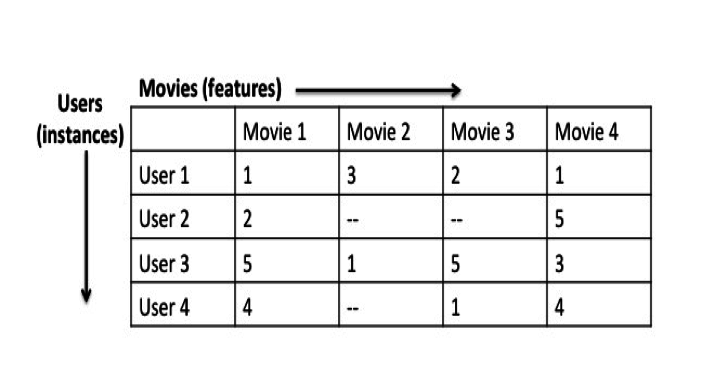
Consider data from a movie rating system where the movie ratings from different users are instances, and the various movies are features.
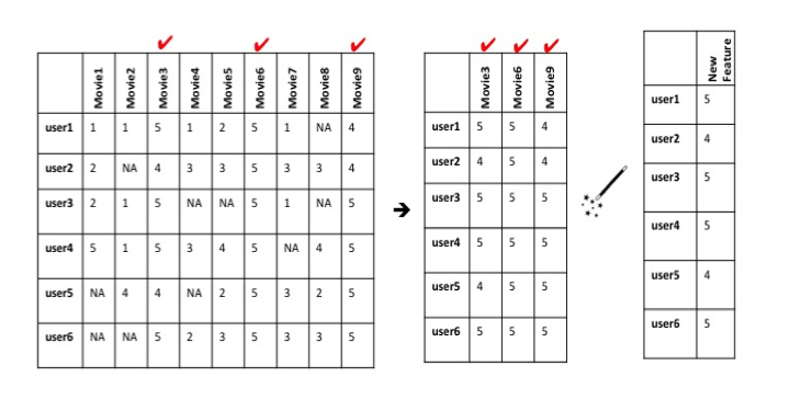
In this dataset, you might observe that users who rank Star Wars Episode IVhighly might also rank Rogue One: A Star Wars Story highly. In other words, the ratings for Star Wars Episode IV are positively correlated with the ones for Rogue One: A Star Wars Story. One could image that all movies ranked by certain users in a similar way might all share similar attributes (ex. all movies with these ratings are classic sci-fi movies), and could ultimately be grouped together to form a new feature.
This is an intuitive way of grouping data, but it would take quite some time to read through all of the data and group it according to similar attributes. Fortunately, there are algorithms that can automatically group features that vary in a similar way within high-dimensional datasets, such as Principal Component Analysis.
The overall goal of PCA is to reduce the number of d dimensions (features) in a dataset by projecting it onto a k dimensional subspace where k < d. The approach used to complete PCA can be summarized as follows:
- Standardize the data.
- Use the standardized data to generate a covariance matrix (or perform Singular Vector Decomposition).
- Obtain eigenvectors (principal components) and eigenvalues from the covariance matrix. Each eigenvector will have a corresponding eigenvalue.
- Sort the eigenvalues in descending order.
- Select the k eigenvectors with the largest eigenvalues, where k is the number of dimensions used in the new feature space (k≤d).
- Construct a new matrix with the selected k eigenvectors.
Tutorial
In this post, we’ll use a high-dimensional movie rating dataset to illustrate how to apply Principal Component Analysis (PCA) to compress the data. This tutorial picks up after having created csv files from the data. If you want to pick up where this tutorial starts, you can find the pre-made csv files here.
Step 1: Load and Standardize Data
First we’ll load the data and store it in a pandas dataframe. The data set contains ratings from 718 users (instances) for 8,913 movies (features). Even though all of the features in the dataset are measured on the same scale (a 0 through 5 rating), we must make sure that we standardize the data by transforming it onto a unit scale (mean=0 and variance=1). Also, all null (NaN) values were converted to 0. It is necessary to transform data because PCA can only be applied on numerical data.
#Load dependencies
import pandas as pd
import numpy as np
from sklearn.preprocessing import StandardScaler
from matplotlib import*
import matplotlib.pyplot as plt
from matplotlib.cm import register_cmap
from scipy import stats
from sklearn.decomposition import PCA as sklearnPCA
import seaborn
#Load movie names and movie ratings
movies = pd.read_csv('movies.csv')
ratings = pd.read_csv('ratings.csv')
ratings.drop(['timestamp'], axis=1, inplace=True)
def replace_name(x):
    return movies[movies['movieId']==x].title.values[0]
ratings.movieId = ratings.movieId.map(replace_name)
M = ratings.pivot_table(index=['userId'], columns=['movieId'], values='rating')
m = M.shape
df1 = M.replace(np.nan, 0, regex=True)
X_std = StandardScaler().fit_transform(df1)
Step 2: Covariance Matrix and Eigendecomposition
Next, a covariance matrix is created based on the standardized data. The covariance matrix is a representation of the covariance between each feature in the original dataset.
The covariance matrix can be found as follows:
mean_vec = np.mean(X_std, axis=0)
cov_mat = (X_std - mean_vec).T.dot((X_std - mean_vec)) / (X_std.shape[0]-1)
print('Covariance matrix \n%s' %cov_mat)
Alternatively, you can also create the same covariance matrix with one line of code.
print('NumPy covariance matrix: \n%s' %np.cov(X_std.T))
Covariance matrix
    [[ 1.0013947  -0.00276421 -0.00195661 ..., -0.00858289 -0.00321221
      -0.01055463]
     [-0.00276421  1.0013947  -0.00197311 ...,  0.14004611 -0.0032393
      -0.01064364]
     [-0.00195661 -0.00197311  1.0013947  ..., -0.00612653 -0.0022929
      -0.00753398]
     ...,
     [-0.00858289  0.14004611 -0.00612653 ...,  1.0013947   0.02888777
       0.14005644]
     [-0.00321221 -0.0032393  -0.0022929  ...,  0.02888777  1.0013947
       0.01676203]
     [-0.01055463 -0.01064364 -0.00753398 ...,  0.14005644  0.01676203
       1.0013947 ]]
    NumPy covariance matrix:
    [[ 1.0013947  -0.00276421 -0.00195661 ..., -0.00858289 -0.00321221
      -0.01055463]
     [-0.00276421  1.0013947  -0.00197311 ...,  0.14004611 -0.0032393
      -0.01064364]
     [-0.00195661 -0.00197311  1.0013947  ..., -0.00612653 -0.0022929
      -0.00753398]
     ...,
     [-0.00858289  0.14004611 -0.00612653 ...,  1.0013947   0.02888777
       0.14005644]
     [-0.00321221 -0.0032393  -0.0022929  ...,  0.02888777  1.0013947
       0.01676203]
     [-0.01055463 -0.01064364 -0.00753398 ...,  0.14005644  0.01676203
       1.0013947 ]]
After the covariance matrix is generated, eigendecomposition is performed on the covariance matrix. Eigenvectors and eigenvalues are found as a result of the eigendceomposition. Each eigenvector has a corresponding eigenvalue, and the sum of the eigenvalues represents all of the variance within the entire dataset.
The eigendecomposition can be performed as follows:
#Perform eigendecomposition on covariance matrix
cov_mat = np.cov(X_std.T)
eig_vals, eig_vecs = np.linalg.eig(cov_mat)
print('Eigenvectors \n%s' %eig_vecs)
print('\nEigenvalues \n%s' %eig_vals)
Step 3: Selecting Principal Components
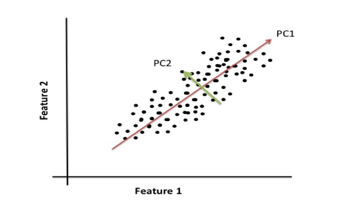
Eigenvectors, or principal components, are a normalized linear combination of the features in the original dataset. The first principal component captures the most variance in the original variables, and the second component is a representation of the second highest variance within the dataset.
For example, if you were to plot data from a dataset that contains two features, the following illustrates that principal component 1 (PC1) represents the direction of the most variation between the two features and principal component 2 (PC2) represents the second most variation between the two plotted features. Our movies dataset contains over 8,000 features and would be difficult to visualize which is why we used eigendecomposition to generate the eigenvectors.
The eigenvectors with the lowest eigenvalues describe the least amount of variation within the dataset. Therefore, these values can be dropped. First, lets order the eigenvalues in descending order:
# Visually confirm that the list is correctly sorted by decreasing eigenvalues
eig_pairs = [(np.abs(eig_vals[i]), eig_vecs[:,i]) for i in range(len(eig_vals))]
print('Eigenvalues in descending order:')
for i in eig_pairs:
    print(i[0])
To get a better idea of how principal components describe the variance in the data, we will look at the explained variance ratio of the first two principal components.
pca = PCA(n_components=2)
pca.fit_transform(df1)
print pca.explained_variance_ratio_
The first two principal components describe approximately 14% of the variance in the data. In order gain a more comprehensive view of how each principal component explains the variance within the data, we will construct a scree plot. A scree plot displays the variance explained by each principal component within the analysis.
#Explained variance
pca = PCA().fit(X_std)
plt.plot(np.cumsum(pca.explained_variance_ratio_))
plt.xlabel('number of components')
plt.ylabel('cumulative explained variance')
plt.show()
Our scree plot shows that the first 480 principal components describe most of the variation (information) within the data. This is a major reduction from the initial 8,913 features. Therefore, the first 480 eigenvectors should be used to construct the dimensions for the new feature space.
Challenge
Try it on your own with a larger data set. What impact do you think a data set with more instances, but similar number of features would have on the resulting number of principal components (our kvalue)? What impact would a dataset with a larger number of features have on the resulting number of principal components?
References
- http://scikit-learn.org/stable/modules/decomposition.html
- http://scikit-learn.org/stable/modules/unsupervised_reduction.html
- Raschka, Sebastian. Principle Component Analysis in 3 Simple Steps, (2015)
- http://www.analyticsvidhya.com/blog/2016/03/practical-guide-principal-component-analysis-python/
- http://support.minitab.com/en-us/minitab/17/topic-library/modeling-statistics/multivariate/principal-components-and-factor-analysis/what-is-a-scree-plot/
- F. Maxwell Harper and Joseph A. Konstan. 2015. The MovieLens Datasets: History and Context. ACM Transactions on Interactive Intelligent Systems (TiiS) 5, 4, Article 19 (December 2015), 19 pages
- https://github.com/databricks/spark-training/tree/master/data/movielens/medium


No comments:
Post a Comment